The details below demonstrate how the models, methods, and techniques of Meta Analysis can be applied via the metafor package.
The Data
The data are provided below and can be loaded with :
library(metafor)
metadat <- read.csv("MetaTest.csv",header = T,sep = ",")
metadat
##    ID                          AUTHOR YEAR        CLASS   OR   LB   UB
## 1   1           Patel et al. (female) 2006   ≥9h vs. 7h 1.03 0.93 1.14
## 2   2                Stranges et al.  2008   ≥9h vs. 7h 0.91 0.27 3.01
## 3   3          Watanabe et al. (male) 2010 ≥9h vs. 7-8h 1.42 0.69 2.96
## 4   4                Nishiura et al.  2010 ≥8h vs. 7-8h 0.75 0.35 1.62
## 5   5     Yiengprugsawan et al. (all) 2012   ≥9h vs. 8h 1.48 0.57 3.83
## 6   6         Sayón-Orea et al. (all) 2013 ≥8h vs. 7-8h 1.30 0.90 1.80
## 7   7                    Nagai et al. 2013   ≥9h vs. 7h 1.06 0.86 1.29
## 8   8 Theorell-Hagl?w et al. (female) 2014   ≥9h vs. 7h 1.12 0.84 1.49
## 9   9 Theorell-Hagl?w et al. (female) 2014   ≥9h vs. 7h 1.13 0.89 1.43
## 10 10 Theorell-Hagl?w et al. (female) 2014   ≥9h vs. 7h 1.52 0.63 3.67
Then we can easily transform these OR values to log odds ratios with:
metadat$yi <- log(metadat$OR)
The confidence interval bounds can be converted into the standard errors with:
metadat$sei <- with(metadat,(log(UB)-log(LB))/(2*1.96))
And thus:
metadat$vi <- metadat$sei^2
metadat
##    ID                          AUTHOR YEAR        CLASS   OR   LB   UB
## 1   1           Patel et al. (female) 2006   ≥9h vs. 7h 1.03 0.93 1.14
## 2   2                Stranges et al.  2008   ≥9h vs. 7h 0.91 0.27 3.01
## 3   3          Watanabe et al. (male) 2010 ≥9h vs. 7-8h 1.42 0.69 2.96
## 4   4                Nishiura et al.  2010 ≥8h vs. 7-8h 0.75 0.35 1.62
## 5   5     Yiengprugsawan et al. (all) 2012   ≥9h vs. 8h 1.48 0.57 3.83
## 6   6         Sayón-Orea et al. (all) 2013 ≥8h vs. 7-8h 1.30 0.90 1.80
## 7   7                    Nagai et al. 2013   ≥9h vs. 7h 1.06 0.86 1.29
## 8   8 Theorell-Hagl?w et al. (female) 2014   ≥9h vs. 7h 1.12 0.84 1.49
## 9   9 Theorell-Hagl?w et al. (female) 2014   ≥9h vs. 7h 1.13 0.89 1.43
## 10 10 Theorell-Hagl?w et al. (female) 2014   ≥9h vs. 7h 1.52 0.63 3.67
##             yi        sei          vi
## 1   0.02955880 0.05193851 0.002697609
## 2  -0.09431068 0.61512076 0.378373556
## 3   0.35065687 0.37149310 0.138007123
## 4  -0.28768207 0.39087966 0.152786910
## 5   0.39204209 0.48596524 0.236162210
## 6   0.26236426 0.17682326 0.031266465
## 7   0.05826891 0.10343498 0.010698794
## 8   0.11332869 0.14620651 0.021376343
## 9   0.12221763 0.12097150 0.014634103
## 10  0.41871033 0.44954774 0.202093166
Modeling
Next, a model can be fitted to these data with:
mod <- rma(yi,vi,data = metadat)
mod
##
## Random-Effects Model (k = 10; tau^2 estimator: REML)
##
## tau^2 (estimated amount of total heterogeneity): 0 (SE = 0.0064)
## tau (square root of estimated tau^2 value):      0
## I^2 (total heterogeneity / total variability):   0.00%
## H^2 (total variability / sampling variability):  1.00
##
## Test for Heterogeneity:
## Q(df = 9) = 4.5909, p-val = 0.8684
##
## Model Results:
##
## estimate       se     zval     pval    ci.lb    ci.ub
##   0.0669   0.0396   1.6876   0.0915  -0.0108   0.1445        .
##
## ---
## Signif. codes:  0 '***' 0.001 '**' 0.01 '*' 0.05 '.' 0.1 ' ' 1
# [Tips] more infirmation can be observed with :
summary(mod)
##
## Random-Effects Model (k = 10; tau^2 estimator: REML)
##
##   logLik  deviance       AIC       BIC      AICc
##   2.2878   -4.5756   -0.5756   -0.1812    1.4244
##
## tau^2 (estimated amount of total heterogeneity): 0 (SE = 0.0064)
## tau (square root of estimated tau^2 value):      0
## I^2 (total heterogeneity / total variability):   0.00%
## H^2 (total variability / sampling variability):  1.00
##
## Test for Heterogeneity:
## Q(df = 9) = 4.5909, p-val = 0.8684
##
## Model Results:
##
## estimate       se     zval     pval    ci.lb    ci.ub
##   0.0669   0.0396   1.6876   0.0915  -0.0108   0.1445        .
##
## ---
## Signif. codes:  0 '***' 0.001 '**' 0.01 '*' 0.05 '.' 0.1 ' ' 1
confint(mod)
##
##        estimate  ci.lb   ci.ub
## tau^2    0.0000 0.0000  0.0287
## tau      0.0000 0.0000  0.1693
## I^2(%)   0.0000 0.0000 55.6963
## H^2      1.0000 1.0000  2.2571
predict(mod,transf = exp)
##    pred  ci.lb  ci.ub  cr.lb  cr.ub
##  1.0692 0.9893 1.1555 0.9893 1.1555
These results shows the amount of heterogeneity (“between-trial variance”) is estimated to be with a standard error of and the I2 = 0, H2 = 1. Since the I2 = 0, the fixed-effect model can be a more appropriate method. And test for heterogeneity is Q = 4.5908637, P−value = 0.8684174,which shows less heterogeneity between thses studies.
Fixed-effect Model
mod <- rma(yi,vi,data = metadat,method = "FE")
mod
##
## Fixed-Effects Model (k = 10)
##
## Test for Heterogeneity:
## Q(df = 9) = 4.5909, p-val = 0.8684
##
## Model Results:
##
## estimate       se     zval     pval    ci.lb    ci.ub
##   0.0669   0.0396   1.6876   0.0915  -0.0108   0.1445        .
##
## ---
## Signif. codes:  0 '***' 0.001 '**' 0.01 '*' 0.05 '.' 0.1 ' ' 1
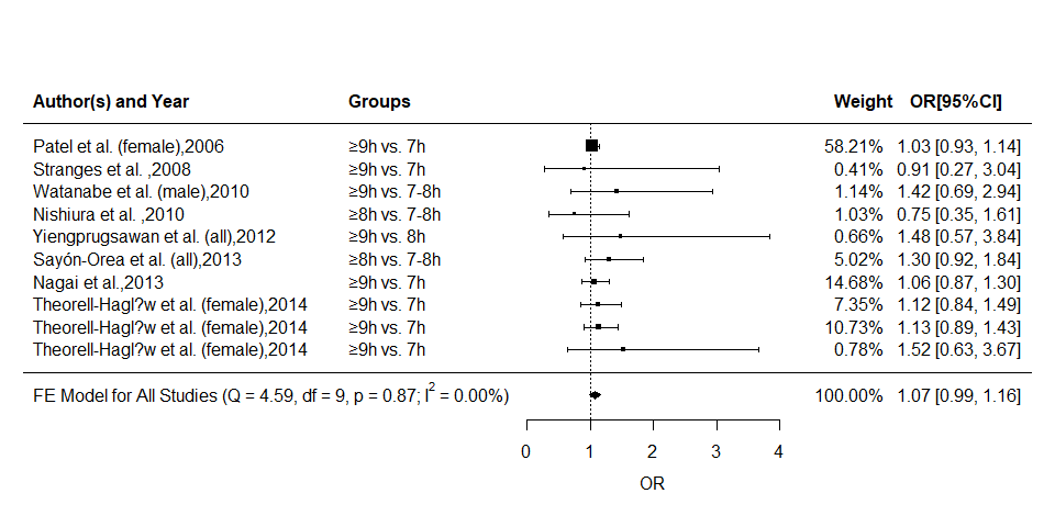
Forest Plot
We can easily plot forest graph with:
forest(mod,transf = exp,refline = 1,
       mlab = "",
       slab = paste(metadat$AUTHOR,metadat$YEAR,sep = ","),
       xlim = c(-8,8),alim = c(0,4),steps = 5,xlab = "OR",
       showweights = T)
#more details added to the figure with text() function
text(-3,10:1,pos = 4,metadat$CLASS)
text(c(-8,-3,4.7,5.9),12,pos = c(4,4,4,4),
     c("Author(s) and Year","Groups","Weight","OR[95%CI]"),
     cex = 1,font = 2)
text(-8,-1,pos = 4,
     bquote(paste("FE Model for All Studies (Q = ",
                  .(formatC(mod$QE,digits = 2,format = "f")),
                  ", df = ",.(mod$k-mod$p),", p = ",
                  .(formatC(mod$QEp,digits = 2,format = "f")),
                  "; ",I^2," = ",
                  .(formatC(mod$I2,digits = 2,format = "f")),
                  "%)")))
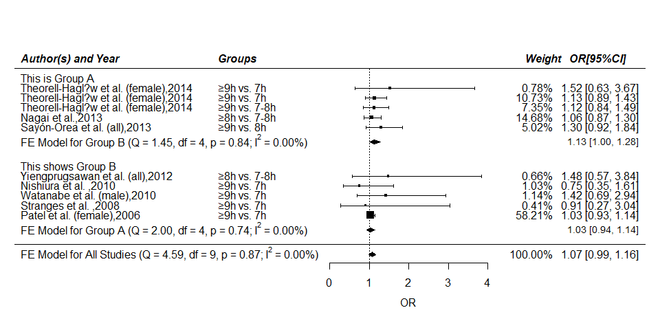
Forest Plot with Subgroups
Description:
Below is an example of a forest plot with two subgroups. The results of the individual studies are shown grouped together according to their subgroup. Below each subgroup, a summary polygon shows the results when fitting a fixed-effects model just to the studies within that group. The summary polygon at the bottom of the plot shows the results from a fixed-effects model when analyzing all 10 studies.
*[Tips] Here we divided the above-mentioned 10 stuies into two groups, Group A = (YEAR <= 2012) vs. Group B = (YEAR > 2012). The grouping approach may have no concrete or practical significance. *
Subgroups Modeling
Fit fixed-effects model in the two subgroups:
mod.a <- rma(yi,vi,data = metadat,subset = (YEAR<=2012),method = "FE")
mod.a
##
## Fixed-Effects Model (k = 5)
##
## Test for Heterogeneity:
## Q(df = 4) = 1.9973, p-val = 0.7363
##
## Model Results:
##
## estimate       se     zval     pval    ci.lb    ci.ub
##   0.0333   0.0505   0.6585   0.5102  -0.0658   0.1324
##
## ---
## Signif. codes:  0 '***' 0.001 '**' 0.01 '*' 0.05 '.' 0.1 ' ' 1
mod.b <- rma(yi,vi,data = metadat,subset = (YEAR> 2012),method = "FE")
mod.b
##
## Fixed-Effects Model (k = 5)
##
## Test for Heterogeneity:
## Q(df = 4) = 1.4483, p-val = 0.8358
##
## Model Results:
##
## estimate       se     zval     pval    ci.lb    ci.ub
##   0.1204   0.0638   1.8867   0.0592  -0.0047   0.2455        .
##
## ---
## Signif. codes:  0 '***' 0.001 '**' 0.01 '*' 0.05 '.' 0.1 ' ' 1
Forest Plot with Subgroups
forest(mod,transf = exp,refline = 1,
       mlab = "",
       slab = paste(metadat$AUTHOR,metadat$YEAR,sep = ","),
       xlim = c(-8,8),alim = c(0,4),steps = 5,xlab = "OR",
       ylim = c(-1,20),order = order(metadat$YEAR),
       rows = c(3:7,12:16),
       showweights = T)

text(-8,-1,pos = 4,
     bquote(paste("FE Model for All Studies (Q = ",
            .(formatC(mod$QE,digits = 2,format = "f")),
            ", df = ",.(mod$k-mod$p),", p = ",
            .(formatC(mod$QEp,digits = 2,format = "f")),
            "; ",I^2," = ",
            .(formatC(mod$I2,digits = 2,format = "f")),
             "%)")))
# add text for the subgroups
text(-8, c(17,8), pos=4, c("This is Group A","This shows Group B"))

# add column headings to the plot
text(-3,c(16:12,7:3),pos = 4,metadat$CLASS)
text(c(-8,-3,4.8,5.9),19,pos = c(4,4,4,4),
     c("Author(s) and Year","Groups","Weight","OR[95%CI]"),
     cex = 1,font = 4)

# add summary polygons for the two subgroups
addpoly(mod.b, row=10.5,  transf=exp, mlab="")
addpoly(mod.a, row= 1.5,  transf=exp, mlab="")

# add text with Q-value, dfs, p-value, and I^2 statistic for subgroups
text(-8,10.5,pos = 4,
     bquote(paste("FE Model for Group B (Q = ",
            .(formatC(mod.b$QE,digits = 2,format = "f")),
            ", df = ",.(mod.b$k-mod.b$p),", p = ",
            .(formatC(mod.b$QEp,digits = 2,format = "f")),
            "; ",I^2," = ",
            .(formatC(mod.b$I2,digits = 2,format = "f")),
            "%)")))
text(-8,1.5,pos = 4,
     bquote(paste("FE Model for Group A (Q = ",
            .(formatC(mod.a$QE,digits = 2,format = "f")),
            ", df = ",.(mod.a$k-mod.a$p),", p = ",
            .(formatC(mod.a$QEp,digits = 2,format = "f")),
            "; ",I^2," = ",
            .(formatC(mod.a$I2,digits = 2,format = "f")),
            "%)")))
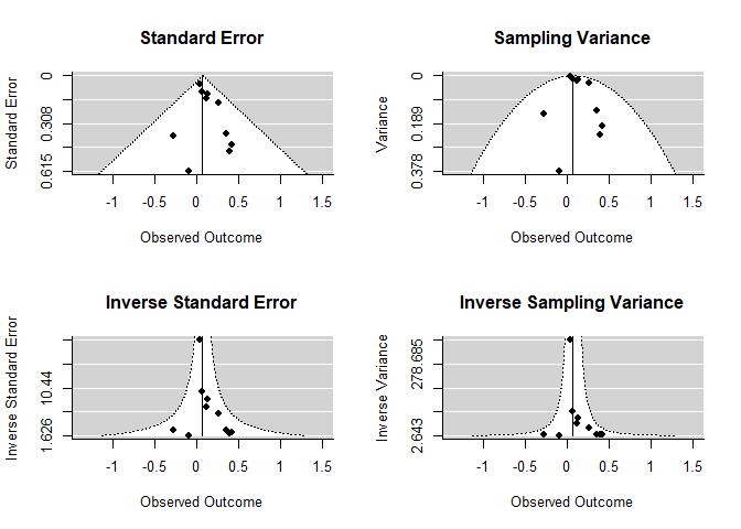
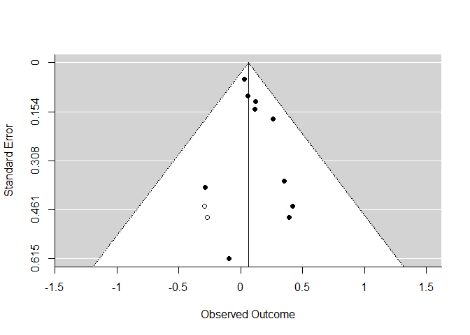
Funnel Plot
par(mfrow=c(2,2))

funnel(mod, main="Standard Error")
funnel(mod, yaxis="vi", main="Sampling Variance")
funnel(mod, yaxis="seinv", main="Inverse Standard Error")
funnel(mod, yaxis="vinv", main="Inverse Sampling Variance")
Egger’s Test
regtest(mod)
##
## Regression Test for Funnel Plot Asymmetry
##
## model:     fixed-effects meta-regression model
## predictor: standard error
##
## test for funnel plot asymmetry: z = 1.0388, p = 0.2989
Sensitivity Analysis
leave1out(mod,transf = exp)
##    estimate   zval   pval  ci.lb  ci.ub      Q     Qp
## 1    1.1262 1.9388 0.0525 0.9987 1.2699 3.3561 0.9101
## 2    1.0699 1.7010 0.0889 0.9898 1.1565 4.5219 0.8072
## 3    1.0657 1.5960 0.1105 0.9856 1.1522 4.0006 0.8571
## 4    1.0731 1.7713 0.0765 0.9925 1.1602 3.7596 0.8781
## 5    1.0668 1.6272 0.1037 0.9869 1.1533 4.1401 0.8443
## 6    1.0582 1.3904 0.1644 0.9771 1.1459 3.3039 0.9139
## 7    1.0707 1.5933 0.1111 0.9844 1.1647 4.5828 0.8011
## 8    1.0652 1.5350 0.1248 0.9827 1.1547 4.4819 0.8112
## 9    1.0621 1.4359 0.1510 0.9783 1.1531 4.3564 0.8236
## 10   1.0662 1.6118 0.1070 0.9862 1.1527 3.9735 0.8595
Funnel Plot with Trim and Fill
taf <- trimfill(mod)
funnel(taf)
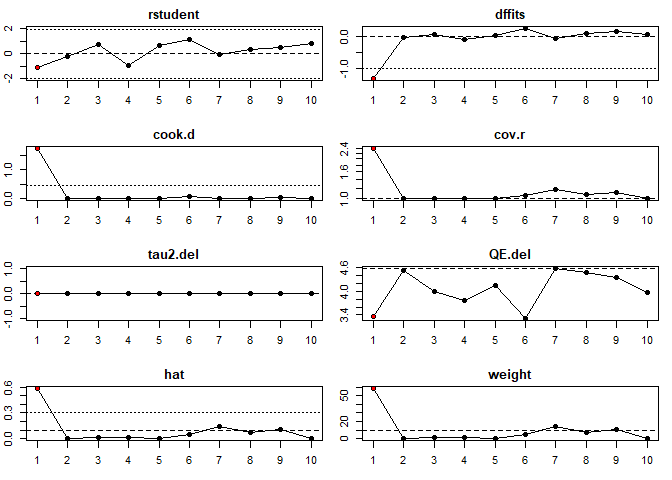
Plot of Influence Diagnostics
inf <- influence(mod)
plot(inf,layout = c(4,2))
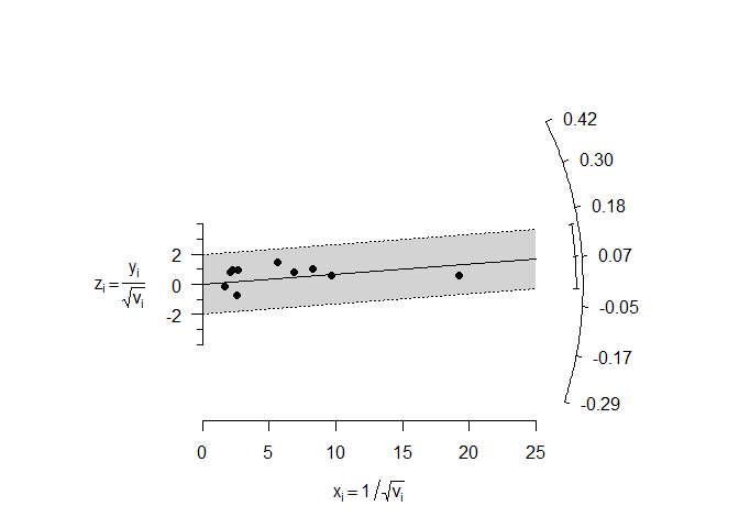
Radial (Galbraith) Plot
Radial plots were introduced by Rex Galbraith (1988a, 1988b, 1994) and can be useful in the meta-analytic context to examine the data for heterogeneity. For a fixed-effects model, the plot shows the inverse of the standard errors on the horizontal axis against the individual observed effect sizes or outcomes standardized by their corresponding standard errors on the vertical axis. On the right hand side of the plot, an arc is drawn corresponding to the individual observed effect sizes or outcomes. A line projected from (0,0) through a particular point within the plot onto this arc indicates the value of the individual observed effect size or outcome for that point. An example of such a plot is shown below.
radial(mod)
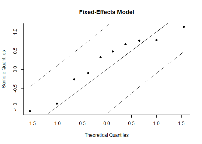
Normal QQ Plots
Normal quantile-quantile (QQ) plots can be useful in meta-analyses to check various aspects and assumptions of the data. Ideally, the points in the plot should fall on a diagonal line with slope of 1, going through the (0,0) point.
qqnorm(mod, main="Fixed-Effects Model")
GOSH Plot
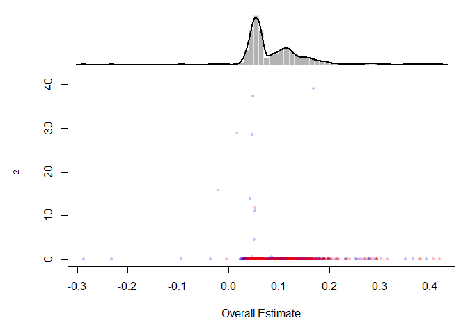
Olkin, Dahabreh, and Trikalinos (2012) proposed the GOSH (graphical display of study heterogeneity) plot, which is based on examining the results of a fixed-effects model in all possible subsets of size 1, …, k of the k studies included in a meta-analysis. In a homogeneous set of studies, the model estimates obtained this way should form a roughly symmetric, contiguous, and unimodal distribution. On the other hand, when the distribution is multimodal, then this suggests the presence of heterogeneity, possibly due to outliers and/or distinct subgroupings of studies. Plotting the estimates against some measure of heterogeneity (e.g. I2, H2, or the Q-statistic) can also help to reveal subclusters, which are indicative of heterogeneity.
Below, a fixed-effects model is first fitted to all trials and then the gosh() function is used to fit fixed-effects models in all possible subsets. The GOSH plot is then created by plotting the results. The points for subsets that include the MetaTest.csv (study 10 in the dataset) are shown in red and blue otherwise.
sav <- gosh(mod)
## Fitting 1023 models (based on all possible subsets).
##
  |
  |                                                                 |   0%
  |
  |                                                                 |   1%
  |
  |=================================================================| 100%
plot(sav, out=10, breaks=100, adjust=0.5, yhist=FALSE, hh=0.2)